Workflow

For full information, please see the latest publication (linked here: Citation).

The workflow and conceptual idea behind diffTF is illustrated by the following three Figures. First, we give a high-level conceptual overview and a biological motivation:

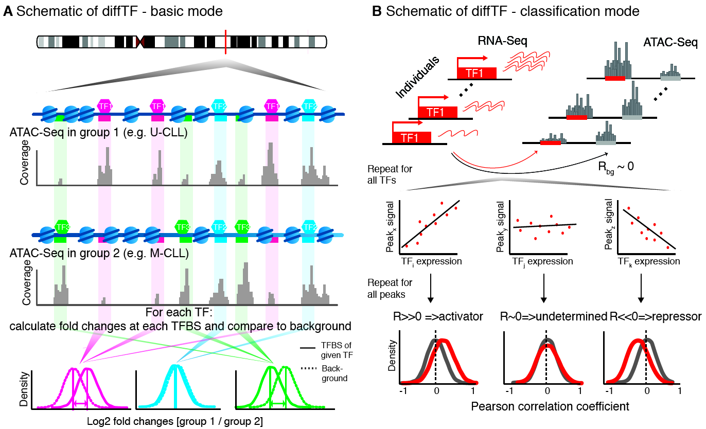
Conceptual idea and workflow of diffTF, the two different modes and the classification

Next, we show a schematic of the diffTF workflow from a more technical perspective by showing the actual steps that are performed:

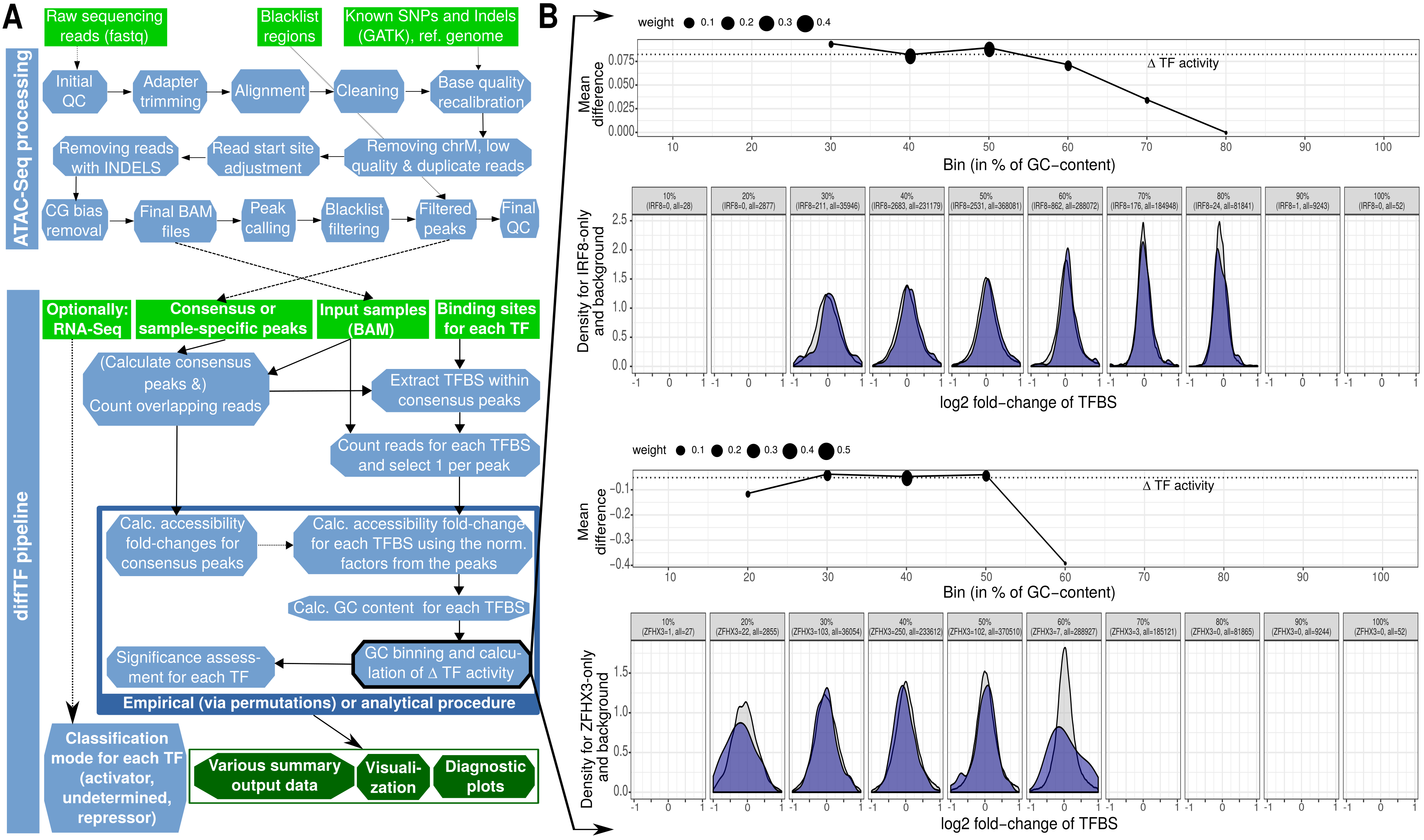
Summary workflows for data processing and methodological details for diffTF (for more details, see Suppl. Figure 1 in the publication).

We now show which rules are executed by Snakemake for a specific example (see the caption of the image):

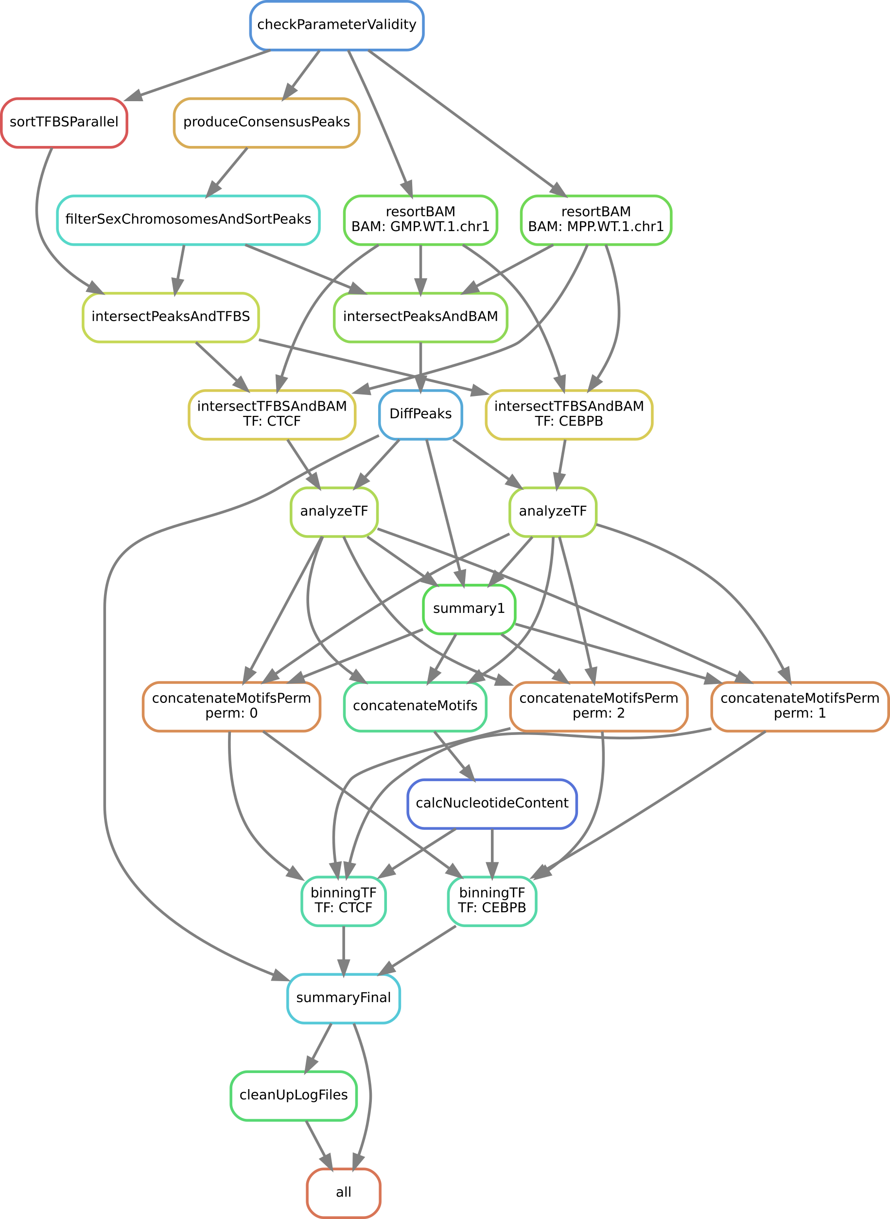
Exact workflow (a so-called directed acyclic graph, or DAG) that is executed when calling Snakemake for an easy of example with two TFs (CEBPB and CTCF) for the two samples GMP.WT1 and MPP.WT1. Each node represents a rule name as defined in the Snakefile, and each arrow a dependency.

diffTF is currently implemented as a Snakemake pipeline. For a gentle introduction about Snakemake, see Section Running diffTF. As you can see, the workflow consists of the following steps or rules:

• checkParameterValidity: R script that checks whether the specified peak file has the correct format, whether the provided fasta file and the BAM files are compatible, and other checks
• produceConsensusPeaks: R script that generates the consensus peaks using the R package DiffBind if none are provided
• filterSexChromosomesAndSortPeaks: Filters various chromosomes (sex, unassembled ones, contigs, etc) from the peak file.
• sortTFBSParallel: Sort the TFBS lists by position
• resortBAM: Sort the BAM file for optimized processing (only run if data are paired-end)
• intersectPeaksAndBAM: Count all reads for peak regions across all input files
• intersectPeaksAndTFBS: Intersect all TFBS with peak regions to retain only TFBS in peak regions
• intersectTFBSAndBAM: Count all reads from all TFBS across all input files in a TF-specific manner
• DiffPeaks: R script that performs a differential accessibility analysis for the peak regions as well as sample permutations
• analyzeTF: R script that performs a TF-specific differential accessibility analysis
• summary1: R script that summarizes the previous script for all TFs
• concatenateMotifs and concatenateMotifsPerm: Concatenates previous results from either real or permuted data (TFBS motives)
• calcNucleotideContent: Calculates the GC content for all TFBS
• binningTF: R script that performs the binning approach in a TF-specific manner
• summaryFinal: R script that summarizes the analysis and calculates final statistics
• cleanUpLogFiles: Cleans up the LOGS_AND_BENCHMARKS directory (mostly relevant if run in cluster mode)

Input

Summary

As input for diffTF for your own analysis, the following data are needed:

• BAM file with aligned reads for each sample (see summaryFile)
• genome reference fasta that has been used to produce the BAM files (see refGenome_fasta)
• Optionally: corresponding RNA-Seq data (see RNASeqCounts)

In addition, the following files are need, all of which we provide already for human hg19, hg38 and mouse mm10:

• TF-specific list of TFBS (see dir_TFBS)
• mapping table (see HOCOMOCO_mapping)

Lastly, some metadata files are needed that specify diffTF-specific and Snakemake-specific parameters. They are explained in detail in the next sections. If this sounds complicated, don’t worry, just take the example analysis, and you will understand within a few minutes what these files are:

• a general configuration file (General configuration file)
• a metadata file for the samples (Input metadata)
• optionally, if run on a cluster, a cluster configuration file (see in particular the Snakemake documentation for details, but we also provide example cluster files as well as Section Running diffTF in a cluster environment)

General configuration file

To run the pipeline, a configuration file that defines various parameters of the pipeline is required.

Note

Please note the following important points:

• the name of this file is irrelevant, but it must be in the right format (JSON) and it must be referenced correctly when calling Snakemake (via the --configfile parameter). We recommend naming it config.json
• neither section nor parameter names must be changed.
• For parameters that specify a path, both absolute and relative paths are possible. We recommend specifying an absolute path. Relative paths must be specified relative to the Snakemake working directory.
• For parameters that specify a directory, there should be no trailing slash.

In the following, we explain all parameters in detail, organized by section names.

SECTION par_general

outdir

Summary

String. Default “output”. Root output directory.

Details

The root output directory where all output is stored.

maxCoresPerRule (optional)

Summary

Integer > 0. Default 16. Maximum number of cores to use for rules that support multithreading. Optional parameter, if missing, set to a default of 4.

Details

This affects currently only rules involving featureCounts - that is, intersectPeaksAndBAM while for rule intersectTFBSAndBAM, the number of cores is hard-coded to 4. When running Snakemake locally, each rule will use at most this number of cores, while in a cluster setting, this value refers to the maximum number of CPUs an individual job / rule will occupy. If the node the job is executed on has fewer nodes, then the maximum number of cores on the node will be taken.

regionExtension

Summary

Integer >= 0. Default 100. Target region extension in base pairs.

Details

Specifies the number of base pairs each target region (from the peaks file) should be extended in both 5’ and 3’ direction.

comparisonType

Summary

String. Default “”.

Details

This parameter helps to organize complex analysis for which multiple different types of comparisons should be done. Set it to a short but descriptive name that summarizes the type of comparison you are making or the types of cells you compare. The value of this parameter appears as prefix in most output files created by the pipeline. It may also be empty.

conditionComparison

Summary

String. Default “”. Specifies the two conditions you want to compare. Only relevant if conditionSummary is specified as a factor.

Details

This parameter is only relevant if conditionSummary is specified as a factor, in which case it specifies the contrast you are making in diffTF. Otherwise, it is ignored. Exactly two conditions have to be specified, comma-separated. For example, if you want to compare GMP and MPP samples, the parameter should be “GMP,MPP”. Both conditions have to be present in the column “conditionSummary” in the sample file table (see summaryFile (summaryFile)).

Note

The order of the two conditions matters. The condition specified first is the reference condition. For the “GMP,MPP” example, all log2 fold-changes will be the log2fc of MPP as compared to GMP. That means that a positive log2 fold-change means it is higher in MPP as compared to GMP. Consequently, the final TF activity (denoted weighted mean difference in the output tables) will have the same directionality. This is also particularly relevant for the allMotifs output file.

designContrast

Summary

String. Default conditionSummary. Design formula for the differential accessibility analysis.

Details

This important parameter defines the actual contrast that is done in the differential accessibility analysis. That is, which groups of samples are being compared? Examples include mutant vs wild type, mutated vs. unmutated, etc. The last element in the formula must always be conditionSummary, which defines the two groups that are being compared or the continuous variable that is used for inferring negative or positive changes, respectively (see parameter designVariableTypes). This name is currently hard-coded and required by the pipeline. Our pipeline allows including additional variables to model potential confounding variables, like gender, batches etc. For each additional variable that is part of the formula, a corresponding and identically named column in the sample summary file must be specified. For example, for an analysis that also includes the batch number of the samples, you may specify this as “~ Treatment + conditionSummary”.

designContrastRNA

Summary

String. Default conditionSummary. Design formula for the RNA-Seq data. Only relevant and needed if parameter (RNASeqIntegration) is set to true. If missing (to increase compatibility with previous versions of diffTF), the default value will be taken.

Details

This important parameter defines the actual contrast that is done in the differential accessibility analysis. That is, which groups of samples are being compared? Examples include mutant vs wild type, mutated vs. unmutated, etc. The last element in the formula must always be conditionSummary, which defines the two groups that are being compared or the continuous variable that is used for inferring negative or positive changes, respectively (see parameter designVariableTypes). This name is currently hard-coded and required by the pipeline. Our pipeline allows including additional variables to model potential confounding variables, like gender, batches etc. For each additional variable that is part of the formula, a corresponding and identically named column in the sample summary file must be specified. For example, for an analysis that also includes the batch number of the samples, you may specify this as “~ Treatment + conditionSummary”.

designVariableTypes

Summary

String. Default conditionSummary:factor. The data types of all elements listed in designContrast (designContrast).

Details

Names must be separated by commas, spaces are allowed and will be eliminated automatically. The data type must be specified with a “:”, followed by either “numeric”, “integer”, “logical”, or “factor”. For example, if designContrast (designContrast) is specified as “~ Treatment + conditionSummary”, the corresponding types might be “Treatment:factor, conditionSummary:factor”. If a data type is specified as either “logical” or “factor”, the variable will be treated as a discrete variable with a finite number of distinct possibilities (something like batch, for example).

Note

Importantly, conditionSummary can either be specified as “factor” or “numeric”/”integer”, which changes the way the results are interpreted and what the log2 fold-changes represent. conditionSummary is usually specified as factor because you want to make a pairwise comparison of exactly two conditions. If conditionSummary is specified as “integer” or “numeric” (i.e., continuous-valued), however, the variable is treated as continuously-scaled, which changes the interpretation of the results: the reported log2 fold change is then per unit of change of that variable. That is, in the final Volcano plot, TFs displayed in the left side have a negative slope per unit of change of that variable, while TFs at the right side have a positive one.

filterChromosomes (optional)

Summary

TODO

Details

TODO

nPermutations

Summary

Integer >= 0. Default 50. The number of random sample permutations.

Details

If set to a value > 0, in addition to the real data, the sample conditions as specified in the sample table will be randomly permuted nPermutations times. This is the recommended way of computing statistical significances for each TF. In this approach, the resulting significance value captures the significance of the effect size (that is, the TF activity) for the real data as compared to permuted one. Note that the maximum number of possible permutations is limited by the number of samples and can be computed with the binomial coefficient n over k. For example, if you have n = 8 samples in total and they split up in the two conditions/groups as k = 5 / k = 3, the total number of permutations is 8 over 5 or 8 over 3 (they are both identical). We generally recommend setting this value to high values such as 1,000. If the value is set to a number higher than the number of possible permutations, it will be adjusted automatically to the maximum number of permutations as determined by the binomial coefficient.

If set to 0, an alternative way of computing significances that is not based on permutations is performed. First, in the CG normalization step, a Welch Two Sample t-test is performed for each bin and the overall significance by treating the T-statistics as z-scores is calculated, which allows to summarize them across the bins and convert them to one p-value per TF. For this conversion of z-scores per bin to p-value an estimate of the variance of the T-scores is approximated (see the publication for details). This procedure reduces the dependency of the p-value on the sample size (since the number of TFBS can range between a few dozen and multiple tens of thousands depending on the TF).

Note

If set to a value > 0, the nBootstraps (nBootstraps) is ignored and can be set to any value.

Note

While using permutations is the recommended approach for assessing statistical significance, in some cases it might be more useful to use the analytical approach: (1) If the number of samples is small or the groups show a very uneven distributions, the total number of possible permutations is also very small and therefore also the permutation-based approach might not accurately assess significance. As a rough guideline, we do not recommend running less than 100 permutations. (2) This approach is usually more stringent than the analytical one. If you have only small differences between the two groups and despite the fact there is no strong signal to capture in the first place, you may want to run the analytical approach instead in such a case.

Note

The permutation-based approach is computationally more expensive than the analytical approach. The running time of the pipeline increases with the number of permutations.

Warning

Do not change the value of this parameter after (parts of) the pipeline have been run, some steps may fail due to this change. If you really need to change the value, rerun the pipeline from the diffPeaks step onwards.

nBootstraps

Summary

Integer >= 0. Default 1,000. The number of bootstrap for estimating the variance of the TF-specific T scores in the CG binning step.

Details

To properly estimate the variance of the T scores for each TF in the CG binning step, we employ a bootstrap approach using the boot library in R with a user-adjustable number of bootstrap replicates (default 1,000), with resampling the bin-specific data and then performing the t-test against the full sample as described above. We then calculate the variance of the bootstrapped T scores for each bin. For more details, see the methods of the publication.

Note

Only relevant if the nPermutations (nPermutations) is set to 0. If both are set to 0, an error is thrown.

Warning

If bootstraps are used, it is recommended to use a reasonable large number. We recommend a value 1,000 and found that higher numbers do not add much benefit but instead only increase running time unnecessarily.

nGCBins

Summary

Integer > 0. Default 10. Number of GC bins for the binning step.

Details

This parameter sets the number of GC bins that are used during the binning step. The default is to split the data into 10 bins (0-10% GC content, 11-20%, …, 91-100%), for each of which the significance is calculated independently (see Methods). Too many bins may result in bins being skipped due to an insufficient number of TFBS for that particular bin and TF, while too few bins may introduce GC-specific biases when summarizing the signal across all TFBS.

TFs

Summary

String. Default “all”. Either “all” or a comma-separated list of TF names of TFs to include. If set to “all”, all TFs that are found in the directory as specified in dir_TFBS (dir_TFBS) will be used.

Details

If the analysis should be restricted to a subset of TFs, list the names of the TF to include in a comma-separated manner here.

Note

For each TF {TF}, a corresponding file {TF}_TFBS.bed needs to be present in the directory that is specified by dir_TFBS (dir_TFBS). The name of the TF can be anything, and from version 1.7 onwards may also contain additional underscores. See the changelog for details. If you run an older version of diffTF, please update the version.

Warning

We strongly recommending running diffTF with as many TF as possible due to our statistical model that we use that compares against a background model.

dir_scripts

Summary

String. The path to the directory where the R scripts for running the pipeline are stored.

Details

Warning

The folder name must be R, and it has to be located in the same folder as the Snakefile.

RNASeqIntegration

Summary

Logical. true or false. Default false. Should RNA-Seq data be integrated into the pipeline?

Details

If set to true, RNA-Seq counts as specified in RNASeqCounts (RNASeqCounts) will be used to classify each TF into either “activator”, “repressor”, “unknown”, or “not-expressed” for the final Volcano plot visualization and the summary table.

debugMode (optional)

Summary

Logical. true or false. Default false. Enable debug mode for R scripts? Only available and supported for diffTF v1.7 or higher (added in May 2020). So far, only R scripts are supported by the debug mode.

Details

If set to true, the debug mode for R scripts is enabled. The typical usage is as follows: If you receive errors when running one of the R scripts, set it to true, restart Snakemake, and you will see a printed message that the debug mode is enabled and a corresponding R session file (.RData) is saved in the LOGS_AND_BENCHMARKS folder. The script then continues running and the error will appear again. Use this file to sent to us for troubleshooting if being asked for. It contains all information necessary to rerun the step on a different PC, and all input files are read in so they are available within R for others.

SECTION samples

summaryFile

Summary

String. Default “samples.tsv”. Path to the sample metadata file.

Details

Path to a tab-separated file that summarizes the input data. See the section Input metadata and the example file for how this file should look like.

pairedEnd

Summary

Logical. true or false. Default true. Is the data paired-end? If single-end, set to false.

Details

Both paired-end and single-end data can be run with diffTF.

SECTION peaks

consensusPeaks

Summary

String. Default “” (empty). Path to the consensus peak file.

Details

If set to the empty string “”, the pipeline will generate a consensus peaks out of the peak files from each individual sample using the R package DiffBind. For this, you need to provide the following two things:

• a peak file for each sample in the metadata file in the column peaks, see the section Input metadata for details.
• The format of the peak files, as specified in peakType (peakType)

If a file is provided, it must be a valid BED file with at least 3 columns:

• tab-separated columns

• no column names in the first row

• Columns 1 to 3:

  1. Chromosome
  2. Start position
  3. End position

• Optional (content for each is ignored and not checked for validity):

  4. Identifier (will be made unique for each if this is not the case already)
  5. Score
  6. Strand

  Warning

  diffTF will take a long time to run if the number of peaks is too high. We recommend having less than 100,000 peaks. If the number of peaks is higher for your analysis, we strongly recommend filtering the peaks beforehand to include only the most relevant peaks.

peakType

Summary

String. Default narrow. File format of the individual, sample-specific peak files. Only relevant if no consensus peak file has been provided (i.e., the consensusPeaks is empty).

Details

Only needed if no consensus peak set has been provided. All individual peak files must be in the same format. We recommend the narrow format (files ending in .narrowPeak) that is a direct output from MACS2, but other formats are supported. See the help for DiffBind dba for a full list of supported formats, the most common ones include:

• bed: .bed file; peak score is in fifth column
• narrow: narrowPeaks file (from MACS2)

minOverlap

Summary

Integer >= 0 or Float between 0 and 1. Default 2. Minimum overlap for peak files for a peak to be considered into the consensus peak set. Corresponds to the minOverlap argument in the dba function of DiffBind. Only relevant if no consensus peak file has been provided (i.e., consensusPeaks, consensusPeaks, is empty).

Details

Only include peaks in at least this many peak sets in the main binding matrix. If set to a value between zero and one, peak will be included from at least this proportion of peak sets. For more information, see the minOverlap argument in the dba function of DiffBind (see here).

SECTION additionalInputFiles

refGenome_fasta

Summary

String. Default ‘hg19.fasta’. Path to the reference genome fasta file.

Details

Warning

You need write access to the directory in which the fasta file is stored, make sure this is the case or copy the fasta file to a different directory. The reason is that the pipeline produces a fasta index file, which is put in the same directory as the corresponding fasta file. This is a limitation of samtools faidx and not our pipeline.

Note

This file has to be in concordance with the input data; that is, the exact same genome assembly version must be used. In the first step of the pipeline, this is checked explicitly, and any mismatches will result in an error.

dir_TFBS

Summary

String. Path to the directory where the TF-specific files for TFBS results are stored.

Details

Each TF {TF} has to have one BED file, in the format {TF}.bed. Each file must be a valid BED6 file with exactly 6 columns, as follows:

1. chromosome
2. start
3. end
4. ID (or sequence)
5. score or any other numeric column
6. strand

For user convenience, we provide such sorted files as described in the publication as a separate download:

• hg19: For a pre-compiled list of 638 human TF with in-silico predicted TFBS based on the HOCOMOCO 10 database and PWMScan for hg19, download this file:
• hg38: For a pre-compiled list of 767 human TF with in-silico predicted TFBS based on the HOCOMOCO 11 database and FIMO from the MEME suite for hg38, download this file:. For a pre-compiled list of 768 human TF with in-silico predicted TFBS based on the HOCOMOCO 11 database and PWMScan for hg38, download this file:
• mm10: For a pre-compiled list of 422 mouse TF with in-silico predicted TFBS based on the HOCOMOCO 10 database and PWMScan for mm10, download this file:

However, you may also manually create these files to include additional TF of your choice or to be more or less stringent with the predicted TFBS. For this, you only need PWMs for the TF of interest and then a motif prediction tool such as FIMO or MOODS. Note that postprocessing of the BED files may be required to make sure the files to use with *diffTF have exactly 6 columns.*

RNASeqCounts

Summary

String. Default “”. Path to the file with RNA-Seq counts.

Details

If no RNA-Seq data is included, set to the empty string “”. Otherwise, if RNASeqIntegration (RNASeqIntegration) is set to true, specify the path to a tab-separated file with raw RNA-Seq counts (i.e., non-negative integer values, see Figure below). We apply some basic filtering for lowly expressed genes and exclude genes with small counts, so there is principally no need for manual filtering unless you want to do so. For guidance, you may want to read Question 4 here.

The first line must be used for labeling the samples, with column names being identical to the sample names as specific in the sample summary table (summaryFile, summaryFile). If you have RNA-Seq data for only a subset of the input samples, this is no problem - the classification will then naturally only be based on the subset. The first column must be named ENSEMBL and it must contain ENSEMBL IDs (e.g., ENSG00000028277) without dots. The IDs are then matched to the IDs from the file as specified in HOCOMOCO_mapping (HOCOMOCO_mapping). For an example of how the count table should look like, check this image: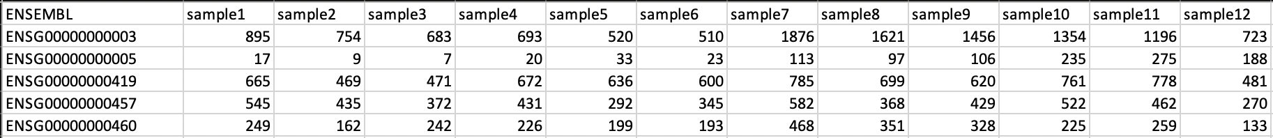

Example of how the RNA-Seq raw count table has to look like. Thanks to Phoebe Valdes for the image and the permission to use it here. Click on the image for better quality.

HOCOMOCO_mapping

Summary

String. Path to the TF-Gene translation table.

Details

If RNA-Seq integration shall be used, a translation table to associate TFs and ENSEMBL genes is needed. For convenience, we provide such a translation table compatible with the pre-provided TFBS lists. Specifically, for each of the currently three TFBS lists, we provide corresponding translation tables for:

1. hg19 with HOCOMOCO 10
2. hg38 with HOCOMOCO 11
3. mm10 with HOCOMOCO 10

If you want to create your own version, check the example translation tables and construct one with an identical structure.

Input metadata

This file summarizes the data and corresponding available metadata that should be used for the analysis. The format is flexible and may contain additional columns that are ignored by the pipeline, so it can be used to capture all available information in a single place. Importantly, the file must be saved as tab-separated, the exact name does not matter as long as it is correctly specified in the configuration file.

Warning

Make sure that the line endings are correct. Different operating systems use different characters to mark the end of line, and the line ending character must be compatible with the operating system in which you run diffTF. For example, if you created the file in MAC, but you run it in a Linux environment (e.g., a cluster system), you may have to convert line endings to make them compatible with Linux. For more information, see here .

It must contain at least contain the following columns (the exact names do matter):

• sampleID: The ID of the sample.

  Note

  Note that each sample ID must be unique! If you want to include replicate samples, rename them, for example by adding “_1”, “_2” etc at the end. All that diffTF cares about is the correct group assignment as defined by the column conditionSummary.

• bamReads: path to the BAM file corresponding to the sample.

  Warning

  All BAM files must meet SAM format specifications. You may use the program ValidateSamFile from the Picard tools to check and identify problems with your file. Chromosome names must have a “chr” as prefix, otherwise diffTF may crash.

• peaks: absolute path to the sample-specific peak file, in the format as given by peakType (peakType). Only needed if no consensus peak file is provided.

• conditionSummary: String with an arbitrary condition name that defines which condition the sample belongs to. There must be only exactly two different conditions across all samples (e.g., mutated and unmutated, day0 and day10, …). In addition, the two conditions must match the ones specified in the conditionComparison (conditionComparison).

• if applicable, all additional variables from the design formula except conditionSummary must also be present as a separate column.

Warning

Do not change the samples data after you started an analysis. You may introduce inconsistencies that will result in error messages. If you need to alter the sample data, we strongly advise to recalculate all steps in the pipeline.

Output

The pipeline produces quite a large number of output files, only some of which are however relevant for the regular user.

Note

In the following, the directory structure and the files are briefly outlined. As some directory or file names depend on specific parameters in the configuration file, curly brackets will be used to denote that the filename depends on a particular parameter or name. For example, {comparisonType} and {regionExtension} refer to comparisonType (comparisonType) and regionExtension ( regionExtension) as specified in the configuration file.

Most files have one of the following file formats:

• .bed.gz (gzipped bed file)
• .tsv.gz (tab-separated value, text file with tab as column separators, gzipped)
• .rds (binary R format, read into with the function readRDS)
• .pdf (PDF format)
• .log (text format)

FOLDER FINAL_OUTPUT

In this folder, the final output files are stored. Most users want to examine the files in here for further analysis.

Sub-folder extension{regionExtension}

Stores results related to the user-specified extension size (regionExtension, regionExtension). In the following, the files are ordered by significance or relevance for interpretation an downstream analyses.

Note

In all output files, in the column permutation, 0 always refers to the non-permuted, real data, while permutations > 0 reflect real permutations.

FILES {comparisonType}.summary.volcano.pdf and {comparisonType}.summary.volcano.q*.pdf

Summary

A visual summary of the results in the form of a Volcano plot. If you run the classification mode, multiple files are created, as follows:

• {comparisonType}.summary.volcano.pdf. This file intentionally empty, see the other files below
• {comparisonType}.summary.volcano.q{X}.pdf, with {X} being 0.001, 0.01, 0.05, and 0.1, corresponding to different stringencies of the classification. Thus, only the classification (i.e, coloring of the data points) differs among the 4 PDF files.

If you run only the basic mode, only the file {comparisonType}.summary.volcano.pdf is created.

Each PDF contains multiple pages, essentially showing the same data but with different filters, and the structure is as follows:

• Basic mode (10 pages in total)
  • Pages 1-5: Volcano plot for different values for the adjusted p-value, starting from the most stringent, 0.001, to 0.01, 0.05, 0.1 and finally the least stringent 0.2
  • Pages 6-10: Same as pages 1-5, just with the raw p-value
• Classification mode (30 pages in total)
  • Pages 1:15: Volcano plot for different values for the adjusted p-value, starting from the most stringent, 0.001, to 0.01, 0.05, 0.1 and finally the least stringent 0.2. For each of these values, 3 pages are shown: 1: all four classes, 2: excluding not-expressed TFs, 3: only showing activator and repressor TFs (see also the legend)
  • Pages 16-30: Same as pages 1-15, just with the raw p-value

Generally, each page shows a Volcano plot of the differential TF activity (labeled as weighted mean difference) between the two conditions you run the analysis for (x-axis) and the corresponding significance (y-axis, adjusted for multiple testing and -log10 transformed). Each point is a TF. The significance threshold is indicated with a dotted line. TFBS is the number of predicted TF binding site that overlap the peak regions and upon which the weighted mean difference is based on. If the classification mode was run, the lgend also shows the TF classification, and points are colored accordingly. Note that different sets of classification classes are shown on each page, see above.

FILE {comparisonType}.summary.tsv.gz

Summary

The final summary table with all diffTF results. This table is also used for the final Volcano plot visualization. The number of columns may vary and depends on the mode you run diffTF for (i.e., only basic mode or also classification mode, analytical or permutation-based approach).

Details

The following columns are always present and relevant:

• TF: name of the TF
• weighted_meanDifference: This is the TF activity value that captures the difference in accessibility between the two conditions. More precisely, it is the difference of the real and background distribution, calculated as the weighted mean across all CG bins (see the publication or Workflow for a graphical depiction of how this works put plot how this is calculated). In the Volcano plot, this is the x-axis. Higher values in either positive and negative direction indicate a larger TF activity in one of the two conditions (i.e., the predicted TF binding sites for this TFs are more accessible). Positive and negative values denote whether the value was bigger in one or the other condition, see the Volcano plot for easier interpretation as well as the notes for :ref:conditionComparison.
• weighted_CD: An alternative measure for the effect size that can be seen as alternative for the weighted_meanDifference but that we provide nevertheless. It is calculated in a similar fashion as the weighted_meanDifference, but instead of taking the difference in the means of the log2 fold-change values from foreground and background, it represents the Cohen’s d measure of effect size (as calculated by the cohensD function from the lsr package), weighted by CG bin as for the weighted_meanDifference.
• TFBS: The number of predicted TF binding sites for the particular TF that overlap with the peaks and that the analysis was based on.
• pvalue: The p-value assesses the significance of the obtained weighted_meanDifference. The exact calculation depends on whether permutations are used (permutation-based approach) or not (analytical approach) and is fully described in the STAR methods of the publication, section “Estimation of significance for differential activity for each TF”
• pvalueAdj: adjusted p-values using Benjamini-Hochberg

The following columns are only relevant if you run the analytical mode:

• weighted_Tstat and variance: These columns are only relevant for the analytical version. See the section “Estimation of significance for differential activity for each TF” in the STAR methods for details. The resulting p-value is based on these columns and we provide them for the sake of completeness.

The following columns are only relevant if you run the classification mode:

• median.cor.tfs: The median value for the RNA-ATAC correlations from the foreground (i.e., peaks with a predicted TFBS for the particular TF)
• classification_*: The columns are explained below, but for each of them, a TF is either classified as activator, undetermined, repressor or not-expressed). For details how TFs are classified, see the STAR methods, section “Classification of TFs into activator and repressors”. Note that the current implementation uses a two-step process to classify TFs. We provide the classifications for both steps for clarity, and they are further subdivided into different classification stringencies (e.g., for more stringent classifications, i.e. smaller values, more TFs are classified as undetermined and only the strongest activators and repressors will be classified as such). These values denote the particular percentiles of the background distribution across the background values for all TF as a threshold for activators and repressors and are used to distinguish real correlations from noise (i.e., activator/repressor from undetermined). The classification stringency goes from 0.001 (most stringent), 0.01, 0.05 to 0.1 (least stringent).
  • classification_q0.* (without final): TF classifications after step 1
  • classification_distr_rawP: The raw p-value of the one-sided Wilcoxon rank sum test for step 2. For TFs that were classified as either repressor or activator after step 1 but for which the raw p value of the Wilcoxon rank sum test was not significant, we changed their classification to undetermined, thereby removing TF classifications with weak support
  • classification_q0.*_final*: TF classifications after step 2 (final, this is what is shown in the Volcano plot)

FILES {comparisonType}.diagnosticPlotsClassification1.pdf and {comparisonType}.diagnosticPlotsClassification2.pdf

Summary

Diagnostic plots related to the classification mode.

File {comparisonType}.diagnosticPlotsClassification1.pdf:

• Pages 1-4: Median Pearson correlation for all TFs, ordered from bottom (lowest) to top (highest). Each dot is one TF, and the color of the dot indicates the TF classification (red: repressor, black/gray: undetermined, green: activator). Each page shows the stringency on which the classification is based for this particular threshold as annotated vertical lines, inside of which TFs are classified as undetermined and outside of it as either repressor (left) or activator (right). The more stringent (i.e., smaller values, see the title), the more the two lines move towards the outside, thereby increasing the width of the “undetermined” area.
• Page 5: Summary density heatmap for each TF and for all classifications across stringencies, sorted by the median Pearson correlation (from the most negative one at the bottom to the most positive one at the top). The heatmap visualizes the correlation across all TFBS, in an alternative representation as compared to the previous pages, summarized in one plot. Colors in or closer to red indicate higher densities and therefore an accumulation of values, while ble or close to blue colors indicate the opposite. Thus, repressors will typically have an enrichment of red colors for negative correlation values, while activators have an enrichment for positive values. TFs will low or conflicting signal will be placed in the middle, classified as undetermined. The left part shows the classification of the TFs for all classification stringencies, sorted from left to right by stringency. The first number refers to the stringency as in other plots and files, but here depicted as per cent (i.e., 0.1% refers to the 0.001 stringency as referred to elsewhere). For each stringency, there are two classifications, referring to the two-step procedure as explained above (columns classification for the file {comparisonType}.summary.tsv.gz). If the signal is strong, the difference between the final and non-final column should be small, while for low-signal classifications, pseudo-significant results will not be significant for the final column.

File {comparisonType}.diagnosticPlotsClassification2.pdf:

• Pages 1-12: Correlation plots of the TF activity (weighted mean differences, x-axis) from the ATAC-Seq for all TF and the log2 fold−changes of the corresponding TF genes from the RNA−seq data (y-axis). Each TF is a point, the size of the point reflects the normalized base mean of the TF gene according to the RNA-Seq data. In addition, the glm regression line is shown, colored by the classification. The correlation plots are shown for different classification stringencies. The title also gives the correlation value for both Pearson and Spearman correlation as well as the corresponding p-values along with the classification stringency
• Page 13-14: Regular (13) and MA plot based shrunken log2 fold-changes (14) of the RNA-Seq counts based on the DESeq2 analysis. Both show the log2 fold changes attributable to a given variable over the mean of normalized counts for all samples, while the latter removes the noise associated with log2 fold changes from low count genes without requiring arbitrary filtering thresholds. Points are colored red if the adjusted p-value is less than 0.1. Points which fall out of the window are plotted as open triangles pointing either up or down. For more information, see here.
• Pages 15-18: Densities of non−normalized (15) and normalized (16) mean log counts for the different samples of the RNA-Seq data, as well their respective empircal cummulative distribution functions (ECDF, pages 17 and 18 for non−normalized and normalized mean log counts, respectively). Since most of the genes are (heavily) affected by the experimental conditions, a successful normalization will lead to overlapping densities. The ECDFs can be thought of as integrals of the densities and give the probability of observing a certain number of counts equal to x or less given the data. For more information, see here.
• Page 19: Mean SD plot (row standard deviations versus row means)
• Page 20-end: Density plots for each TF, with one TF per page. The density plot shows the foreground (red, labeled as Motif) comprising of the log2 fold-changes of all predicted TF binding sites (TFBS, see title) for the particular TF only, while the background (gray, labeled as Non-Motif) shows the log2 fold-changes of all predicted TF binding sites for all other TF.

For the other plots, already documented? To further assess systematic differences between the samples, we can also plot pairwise mean–average plots: We plot the average of the log–transformed counts vs the fold change per gene for each of the sample pairs.

FILE {comparisonType}.diagnosticPlots.pdf

Summary

Various diagnostic plots for the final TF activity values, mostly related to the permutation-based approach.

Details

If the permutation-based approach has been used, the structure is as follows:

• Page 1: Density plot of the weighted mean difference (TF activity) values from the permutations (black) and the real values (red) across all TF. Note that the number of points in the permuted data contains more values - if 1000 permutations have been used for 640 TF, it contains 640 * 1000 values, while the red distribution only contains 640 values. This plot summaries the overall signal: if the red and black curve show little difference, it generally indicates that the observed weighted mean difference (TF activity) values across all TF are very similar to permuted values and therefore, noise. Importantly, however, there might well be individual TFs that show a large signal, which should be visible also in the red line by having outlier values towards the more extreme values. Permuted values, however, usually cluster strongly around 0, which is the expected difference between the conditions if the data are permuted.
• Page 2 onward: Density plot for the weighted mean difference (TF activity) values from the permutations (one value per permutation, black) vs the single real value (red vertical line). The significance that is shown in the Volcano plot is based on the comparison of the permuted vs the real value (see methods for details). In brief, it is calculated as an empirical two-sided p-value per TF by comparing the real value with the distribution from the permutations and calculating the proportion of permutations for which the absolute differential TF activity is larger. For example, the p-value is small if the real value (i.e., the red line) is outside of the distribution or close to the corner of the permuted values. The p-value is consequently large, however, if the real value falls well within the distribution of the permuted values.
• Rest: Various summary plots for different variables

If the analytical mode has been run, the plots related to the permutations are missing from the PDF.

FILE {comparisonType}.allMotifs.tsv.gz

Summary

Summary table for each TFBS. This file contains summary data for each TF and each TFBS and allows a more in-depth investigation.

Details

Columns are as follows:

• permutation: Permutation number. This is always 0 and can therefore be ignored
• TF: name of the TF
• chr, MSS, MES, strand, TFBSID: Genomic location and identifier of the (extended) TFBS
• peakID: Genomic location and annotation of the overlapping peak region
• l2FC, pval, pval_adj: Results from the limma or DESeq2 analysis, see the respective documentation for details (see below for links and further explanation). These column names are shared between limma and DESeq2. l2FC are interpreted as described in the conditionComparison ( conditionComparison)
• DESeq_baseMean, DESeq_ldcSE, DESeq_stat: Results from the DESeq2 analysis, see the DESeq2 documentation for details (e.g., ?DESeq2::results). If DESeq2 was not run for calculating log2 fold-changes (i.e., if the value for the nPermutations ( regionExtension) is >0), these columns are set to NA.
• limma_avgExpr, limma_B, limma_t_stat: Results from the limma analysis, see the limma documentation for details (e.g., ??topTable). If limma was not run (i.e., if the value for the nPermutations ( regionExtension) is 0), these columns are set to NA.

FILE {comparisonType}.TF_vs_peak_distribution.tsv.gz

Summary

This summary table contains various results regarding TFs, their log2 fold change distribution across all TFBS and differences between all TFBS and the peaks

Details

See the description of the file {TF}.{comparisonType}.summary.rds. This file aggregates the data for all TF and adds the following additional columns: - pvalue_adj: adjusted (fdr aka BH) p-value (based on pvalue_raw) - Diff_mean, Diff_median, Diff_mode, Diff_skew: Difference of the mean, median, mode, and skewness between the log2 fold-change distribution across all TFBS and the peaks, respectively

FOLDER PEAKS

Stores peak-associated files.

FILES {comparisonType}.consensusPeaks.filtered.sorted.bed

Summary

Produced in rule filterSexChromosomesAndSortPeaks. Filtered and sorted consensus peaks (see below). the diffTF analysis is based on this set of peaks.

Details

Filtered consensus peaks (removal of peaks from one of the following chromosomes: chrX, chrY, chrM, chrUn*, and all contig names that do not start with “chr” such as *random* or *hap|_gl*

FILE {comparisonType}.allBams.peaks.overlaps.bed.gz

Summary

Produced in rule intersectPeaksAndBAM. Counts for each consensus peak with each of the input BAM files.

Details

No further details provided yet. Please let us know if you need more details.

FILE {comparisonType}.sampleMetadata.rds

Summary

Produced in rule DiffPeaks. Stores data for the input data (similar to the input sample table), for both the real data and the permutations.

Details

No further details provided yet. Please let us know if you need more details.

FILE {comparisonType}.peaks.rds

Summary

Produced in rule DiffPeaks. Internal file. Stores all peaks that will be used in the analysis in rds format.

Details

No further details provided yet. Please let us know if you need more details.

FILE {comparisonType}.peaks.tsv.gz

Summary

Produced in rule DiffPeaks. Stores the results of the differential accessibility analysis for the peaks.

Details

No further details provided yet. Please let us know if you need more details.

FILE {comparisonType}.normFacs.rds

Summary

Produced in rule DiffPeaks. Gene-specific normalization factors for each sample and peak.

Details

This file is produces after the differential accessibility analysis for the peaks. The normalization factors are used for the TF-specific differential accessibility analysis.

FILES {comparisonType}.diagnosticPlots.peaks.pdf

Summary

Produced in rule DiffPeaks. Various diagnostic plots for the differential accessibility peak analysis for the real data.

Details

The pages are as follows:

(1) Density plots of non-normalized (page 1) and normalized (page 2) mean log counts as well their respective empirical cumulative distribution functions (ECDF, pages 3 and 4 for non−normalized and normalized mean log counts, respectively) - Page 5-6: Regular (5) and MA plot based shrunken log2 fold-changes (6) of the RNA-Seq counts based on the DESeq2 analysis for the peaks (not the TF binding sites). Both show the log2 fold changes attributable to a given variable over the mean of normalized counts for all samples, while the latter removes the noise associated with log2 fold changes from low count genes without requiring arbitrary filtering thresholds. Points are colored red if the adjusted p-value is less than 0.1. Points which fall out of the window are plotted as open triangles pointing either up or down. For more information, see here. (2) Page 7 onward: pairwise mean-average plots (average of the log-transformed counts vs the fold-change per peak) for each of the sample pairs. This can be useful to further assess systematic differences between the samples. Note that only a maximum of 20 different pairwise plots are shown for time and efficacy reasons. (3) Last page: mean SD plots (row standard deviations versus row means)

FILE {comparisonType}.DESeq.object.rds

Summary

Produced in rule DiffPeaks. The DESeq2 object from the differential accessibility peak analysis.

Details

No further details provided yet. Please let us know if you need more details.

FOLDER TF-SPECIFIC

Stores TF-specific files. For each TF {TF}, a separate sub-folder {TF} is created by the pipeline. Within this folder, the following structure is created:

Sub-folder extension{regionExtension}

FILES {TF}.{comparisonType}.allBAMs.overlaps.bed.gz and {TF}.{comparisonType}.allBAMs.overlaps.bed.summary

Summary

Overlap and featureCounts summary file of read counts across all TFBS for all input BAM files.

Details

For more details, see the documentation of featureCounts.

FILE {TF}.{comparisonType}.output.tsv.gz

Summary

Produced in rule analyzeTF. A summary table for the differential accessibility analysis.

Details

See the file {comparisonType}.allMotifs.tsv.gz in the FINAL_OUTPUT folder for a column description.

FILE {TF}.{comparisonType}.outputPerm.tsv.gz

Summary

Produced in rule analyzeTF. A subset of the file {TF}.{comparisonType}.output.tsv.gz that stores only the necessary permutation-specific results for subsequent steps.

Details

This file has the following columns (see the description for the file {TF}.{comparisonType}.output.tsv.gz for details): - TF - TFBSID - log2fc_perm columns, which store the permutation-specific log2 fold-changes of the particular TFBS. Permutation 0 refers to the real data

FILE {TF}.{comparisonType}.summary.rds

Summary

Produced in rule analyzeTF. A summary table for the log2 fold-changes across all TFBS limma results.

Details

This file summarizes the TF-specific results for the differential accessibility analysis and has the following columns: - TF: name of the TF - permutation: The number of the permutation. - Pos_l2FC, Mean_l2FC, Median_l2FC, sd_l2FC, Mode_l2FC, skewness_l2FC: fraction of positive values, mean, median, standard deviation, mode value and Bickel’s measure of skewness of the log2 fold change distribution across all TFBS - pvalue_raw and pvalue_adj: raw and adjusted (fdr aka BH) p-value of the t-test - T_statistic: the value of the T statistic from the t-test - TFBS_num: number of TFBS

FILES {TF}.{comparisonType}.diagnosticPlots.pdf

Summary

Produced in rule analyzeTF. Various diagnostic plots for the differential accessibility TFBS analysis for the real data.

Details

See the description of the file {comparisonType}.diagnosticPlots.peaks.pdf in the PEAKS folder, which has an identical structure. Here, the second last page shows two density plots of the log2 fold-changes for the specific pairwise comparson that diffTF run for, one for the peak log2 fold-changes (independent of any TF) and one for the TF-specific one (i.e., across all TFBS from the subset of peaks with a TFBS for this TF). The last page shows the same but in a cumulative representation.

FILE {TF}.{comparisonType}.permutationResults.rds

Summary

Produced in rule binningTF. Contains a data frame that stores the results of bin-specific results.

Details

No further details provided yet. Please let us know if you need more details.

FILE {TF}.{comparisonType}.permutationSummary.tsv.gz

Summary

Produced in rule binningTF. A final summary table that summarizes the results across bins by calculating weighted means.

Details

The data of this table are used for the final visualization.

FILE {TF}.{comparisonType}.covarianceResults.rds

Summary

Produced in rule binningTF. Contains a data frame that stores the results of the pairwise bin covariances and the bin-specific weights.

Details

Note

Covariances are only computed for the real data but not the permuted ones.

FOLDER LOGS_AND_BENCHMARKS

Stores various log and error files.

• *.log files from R scripts: Each log file is produced by the corresponding R script and contains debugging information as well as warnings and errors:
  • checkParameterValidity.R.log
  • produceConsensusPeaks.R.log
  • diffPeaks.R.log
  • analyzeTF.{TF}.R.log for each TF {TF}
  • summary1.R.log
  • binningTF.{TF}.log for each TF {TF}
  • summaryFinal.R.log
• *.log summary files: Summary logs for user convenience, produced at very end of the pipeline only. They should contain all errors and warnings from the pipeline run.
  • all.errors.log
  • all.warnings.log

FOLDER TEMP

Stores temporary and intermediate files. Since they are usually not relevant for the user, they are explained only very briefly here.

Sub-folder SortedBAM

Stores sorted versions of the original BAMs that are optimized for fast count retrieval using featureCounts. Only present if data are paired-end.

• {basenameBAM}.bam for each input BAM file: Produced in rule resortBAM. Resorted BAM file

Sub-folder extension{regionExtension}

Stores results related to the user-specified extension size (regionExtension, regionExtension)

• {comparisonType}.allTFBS.peaks.bed.gz: Produced in rule intersectPeaksAndTFBS. BED file containing all TFBS from all TF that overlap with the peaks after motif extension
• conditionComparison.rds: Produced in rule DiffPeaks. Stores the condition comparison as a string. Some steps in diffTF need this file as input.
• {comparisonType}.motifs.coord.permutation{perm}.bed.gz and {comparisonType}.motifs.coord.nucContent.permutation{perm}.bed.gz for each permutation {perm}: Produced in rule calcNucleotideContent, and needed subsequently for the binning. Temporary and result file of bedtools nuc, respectively. The latter contains the GC content for all TFBS.
• {comparisonType}.checkParameterValidity.done: temporary flag file
• {TF}_TFBS.sorted.bed for each TF {TF}: Produced in rule sortTFBSParallel. Coordinate-sorted version of the input TFBS. Only “regular” chromosomes starting with “chr” are kept, while sex chromosomes (chrX, chrY), chrM and unassembled contigs such as chrUn are additionally removed.
• {comparisonType}.allTFBS.peaks.bed.gz: Produced in rule intersectPeaksAndTFBS. BED file containing all TFBS from all TF that overlap with the peaks before motif extension

Running diffTF

General remarks

diffTF is programmed as a Snakemake pipeline. Snakemake is a bioinformatics workflow manager that uses workflows that are described via a human readable, Python based language. It offers many advantages to the user because each step can easily be modified, parts of the pipeline can be rerun, and workflows can be seamlessly scaled to server, cluster, grid and cloud environments, without the need to modify the workflow definition or only minimal modifications. However, with great flexibility comes a price: the learning curve to work with the pipeline might be a bit higher, especially if you have no Snakemake experience. For a deeper understanding and troubleshooting errors, some knowledge of Snakemake is invaluable.

Simply put, Snakemake executes various rules. Each rule can be thought of as a single recipe or task such as sorting a file, running an R script, etc. Each rule has, among other features, a name, an input, an output, and the command that is executed. You can see in the Snakefile what these rules are and what they do. During the execution, the rule name is displayed, so you know exactly at which step the pipeline is at the given moment. Different rules are connected through their input and output files, so that the output of one rule becomes the input for a subsequent rule, thereby creating dependencies, which ultimately leads to the directed acyclic graph (DAG) that describes the whole workflow. You have seen such a graph in Section Workflow.

In diffTF, a rule is typically executed separately for each TF. One example for a particular rule is sorting the TFBS list for the TF CTCF.

In diffTF, the total number of jobs or rules to execute can roughly be approximated as 3 * nTF, where nTF stands for the number of TFs that are included in the analysis. For each TF, three sets of rules are executed:

1. Calculating read counts for each TFBS within the peak regions (rule intersectTFBSAndBAM)
2. Differential accessibility analysis (rule analyzeTF)
3. Binning step (rule binningTF)

In addition, one rule per permuation is executed, so an additional nPermutations rules are performed. Lastly, a few other rules are executed that however do not add up much more to the overall rule count.

Executing diffTF - Running times and memory requirements

diffTF can be computationally demanding depending on the sample size and the number of peaks. In the following, we discuss various issues related to time and memory requirements and we provide some general guidelines that worked well for us.

Warning

We generally advise to run diffTF in a cluster environment. For small analysis, a local analysis on your machine might work just fine (see the example analysis in the Git repository), but running time increases substantially due to limited amount of available cores.

Analysis size

We now provide a very rough classification into small, medium and large with respect to the sample size and the number of peaks:

• Small: Fewer than 10-15 samples, number of peaks not exceeding 50,000-80,000, normal read depth per sample
• Large: Number of samples larger than say 20 or number of peaks clearly exceeds 100,000, or very high read depth per sample
• Medium: Anything between small and large

Memory

Some notes regarding memory:

• Disk space: Make sure you have enough space left on your device. As a guideline, analysis with 8 samples need around 12 GB of disk space, while a large analysis with 84 samples needs around 45 GB. The number of permutations also has an influence on the (temporary) required storage and a high number of permutations (> 500) may substantially increase the memory footprint. Note that most space is occupied in the TEMP folder, which can be deleted after an analysis has been run successfully. We note, however, that rerunning (parts of) the analysis will require regenerating files from the TEMP folder, so only delete the folder or files if you are sure that you do not need them anymore.
• Machine memory: Although most steps of the pipeline have a modest memory footprint of less than 4 GB or so, depending on the analysis size, some may need 10+ GB of RAM during execution. We therefore recommend having at least 10 GB available for large analysis (see above).

Number of cores

Some notes regarding the number of available cores:

• diffTF can be invoked in a highly parallelized manner, so the more CPUs are available, the better.
• you can use the --cores option when invoking Snakemake to specify the number of cores that are available for the analysis. If you specify 4 cores, for example, up to 4 rules can be run in parallel (if each of them occupies only 1 core), or 1 rule can use up to 4 cores.
• we strongly recommend running diffTF in a cluster environment due to the massive parallelization. With Snakemake, it is easy to run diffTF in a cluster setting. Simply do the following:
  • write a cluster configuration file that specifies which resources each rule needs. For guidance and user convenience, we provide different cluster configuration files for a small and large analysis. See the folder src/clusterConfigurationTemplates for examples. Note that these are rough estimates only. See the *Snakemake* documentation for details for how to use cluster configuration files.
  • invoke Snakemake with one of the available cluster modes, which will depend on your cluster system. We used --cluster and tested the pipeline extensively with LSF/BSUB and SLURM. For more details, see the *Snakemake* documentation

Total running time

Some notes regarding the total running time:

• the total running time is very difficult to estimate beforehand and depends on many parameters, most importantly the number of samples, their read depth, the number of peaks, and the number of TF included in the analysis.
• for small analysis such as the example analysis in the Git repository, running times are roughly 30 minutes with 2 cores for 50 TF and a few hours with all 640 TF.
• for large analysis, running time will be up to a day or so when executed on a cluster machine

Running diffTF in a cluster environment

If diffTF should be run in a cluster environment, the changes are minimal due to the flexibility of Snakemake. You only need to change the following:

• create a cluster configuration file in JSON format. See the files in the clusterConfigurationTemplates folder for examples. In a nutshell, this file specifies the computational requirements and job details for each job that is run via Snakemake.

• invoke Snakemake with a cluster parameter. As an example, you may use the following for a SLURM cluster:

  snakemake -s path/to/Snakefile \
  --configfile path/to/configfile --latency-wait 30 \
  --notemp --rerun-incomplete --reason --keep-going \
  --cores 16 --local-cores 1 --jobs 400 \
  --cluster-config path/to/clusterconfigfile \
  --cluster " sbatch -p {cluster.queue} -J {cluster.name} \
      --cpus-per-task {cluster.nCPUs} \
     --mem {cluster.memory} --time {cluster.maxTime} -o \"{cluster.output}\" \
     -e \"{cluster.error}\"  --mail-type=None --parsable "
  

• the corresponding cluster configuration file might look like this:

  {
    "__default__": {
      "queue": "htc",
      "nCPUs": "{threads}",
      "memory": 2000,
      "maxTime": "1:00:00",
      "name": "{rule}.{wildcards}",
      "output": "{rule}.{wildcards}.out",
      "error": "{rule}.{wildcards}.err"
    },
    "resortBAM": {
      "memory": 5000,
      "maxTime": "1:00:00"
    },
    "intersectPeaksAndPWM": {
      "memory": 5000,
      "maxTime": "1:00:00"
    },
    "intersectPeaksAndBAM": {
      "memory": 5000,
      "maxTime": "1:00:00"
    },
    "intersectTFBSAndBAM": {
      "memory": 5000,
      "maxTime": "1:00:00"
    },
    "DiffPeaks": {
      "memory": 5000,
      "maxTime": "1:00:00"
    },
    "analyzeTF": {
      "memory": 5000,
      "maxTime": "1:00:00"
    },
    "binningTF": {
      "memory": 5000,
      "maxTime": "1:00:00"
    },
    "summaryFinal": {
      "memory": 5000,
      "maxTime": "0:30:00"
    },
    "cleanUpLogFiles": {
      "memory": 1000,
      "maxTime": "0:30:00"
    }
  }
  

A few motes might help you to get started:

• each name in the --cluster argument string from the command line (here: queue, name nCPUs, memory, maxTime, output, and error) must appear also in the __default__ section of the referenced cluster configuration file (via --cluster-config)

• for brevity here, only rules with requirements different from the specified default have been included here in the online version, while the templates in the repository contain all rules, even if they have the same requirements as the default. The latter makes it easier for practical purposes to change requirements later on

• the --cluster argument is the only part that has to be adjusted for your cluster system. It is quite simple really, you essentially just link the content of the configuration file to the cluster system you want to submit the jobs to. More specifically, you refer to the cluster configuration file via the cluster. string, followed by the name of the parameter in the cluster configuration. For parameters that refer to filenames, an extra escaped quotation mark \" has been added so that the command also works in case of spaces in filenames (which should always be avoided at all costs)

• the cluster configuration file has multiple sections defined that correspond to the names of the rules as defined in the Snakefile, plus the special section __default__ at the very top, the latter of which specifies the default cluster options that apply to all rules unless overwritten via its own rule-specific section

• each name (e.g., here: queue, name nCPUs, `memory, maxTime, output, and error) must be defined in the __default__ section of the cluster configuration file

• note that in this example, we provided some extra parameters for convenience such as name (so the cluster job will have a reasonable name and can be recognized) that are not strictly necessary

• the {threads} syntax of the nCPUs name can be generally used and is a placeholder for the specified number of threads for the particular rule, as specified in the corresponding Snakefile

• in our example, memory is given in Megabytes, so 5000 refers to roughly 5 GB. Queue names are either htc or 1day. Adjust this accordingly to your cluster system.

• for more details, see the Snakemake documentation

• Note

  From a practical point of view, just try to mimic the parameters that you usually use for your cluster system, and modify the cluster configuration file accordingly. For example, if you need an additional argument such as -A (which stands for the group you are in for a SLURM-based system), simply add -A {cluster.group} to the command line call and add a group parameter to the __default__ section (see also the note below).

Frequently asked questions (FAQs)

Here a few typical use cases, which we will extend regularly in the future if the need arises:

1. I received an error, and the pipeline did not finish.

As explained in Section Handling errors, you first have to identify and fix the error. Rerunning then becomes trivially easy: just restart Snakemake, it will start off where it left off: at the step that produced that error.

2. I received an error, and I do not see any error message.

First, check the cluster output and error files if you run diffTF in cluster mode. They mostly contain an actual error message or at least the print the exact command that resulted in an error. If you executed locally or still cannot find the error message, see below for guidelines.

3. I want to rerun a specific part of the pipeline only.

This common scenario is also easy to solve: Just invoke Snakemake with --forcerun {rulename}, where {rulename} is the name of the rule as defined in the Snakefile. Snakemake will then rerun the specified run and all parts downstream of the rule. If you want to avoid rerunning downstream parts (think carefully about it, as there might be changes from the rerunning that might have consequences for downstream parts also), you can combine --forcerun with --until and specify the same rule name for both.

4. I want to modify the workflow.

Simply add or modify rules to the Snakefile, it is as easy as that.

5. diffTF finished successfully, but nothing is significant.

This can and will happen, depending on the analysis. The following list provides some potential reasons for this:

• The two conditions are in fact very similar and there is no signal that surpasses the significance threshold. You could, for example, check in a PCA plot based on the peaks that are used as input for diffTF whether they show a clear signal and separation.
• There is a confounding factor (like age) that dilutes the signal. One solution is to add the confounding variable into the design model, see above fo details. Again, check in a PCA plot whether samples cluster also according to another variable.
• You have a small number of samples or one of the groups contains a small number of samples. In both cases, if you run the permutation-based approach, the number of permutations is small, and there might not be enough permutations to achieve significance. For example, if you run an analysis with only 10 permutations, you cannot surpass the 0.05 significance threshold. As a solution, you may switch to the analytical version. Be aware that this requires to rerun large parts of the pipeline from the diffPeaks step onwards.
• You have a very small number of peaks and therefore also a small number of TF binding sites within the peaks, resulting in many TFs to be skipped in the analysis due to an insufficient number of binding sites. As a solution, try increasing the number of peaks or verify that the predicted binding sites are not too stringent (if done independently, therefore not using our TFBS collection that was produced with PWMScan and HOCOMOCO). We recommend having at least a few thousand peaks, but this can hardly be generalized and depends too much on the biology, the size of the peaks etc.
• You run the (usually more stringent) permutation-based approach. If the number of permutations is too low, p-values may not be able to reach significance. For more details, see nPermutations. You may want to rerun the analysis using the analytical approach or using more permutations (if the number of samples makes this possible at all); however, the problems raised above may still apply.

6. diffTF finished successfully, but almost everything is significant.

This can also happen and is usually a good sign. The following list provides some potential reasons for this:

• If you run the analytical mode, consider running the permutation-based approach in addition. The permutation-based approach tends to be more stringent and usually results in fewer TFs being significant. However, as explained in the paper and here, it can only be used if the number of samples is sufficiently high.
• If too many TFs are significant, you have multiple choices that can of course also be combined: First, you may use a more stringent adjusted p-value threshold. Keep in mind that the Volcano plot PDF shows only a few selected thresholds, and you can always be even more stringent when working with the final result table that is also written to the FINAL_OUTPUT folder. Second, you may further filter them by additional criteria such as the number of binding sites (e.g., filtering TFs with a very small number of binding sites, a TF activity that is not large enough, or by their predicted mode of action if you used the classification mode). Third, you may further subdivide them into families and subsequently focus, for example, only one particular TF family. Alternatively, you can classify the TFs into “known” and “novel” for the particular comparison.

7. I want to change the value of a parameter.

If you want to do this, please contact us, and we help and then update the FAQ here.

If you feel that a particular use case is missing, let us know and we will add it here!

Handling errors

Error types

Errors occur during the Snakemake run can principally be divided into:

• Temporary errors (often when running in a cluster setting)
  • might occur due to temporary problems such as bad nodes, file system issues or latencies
  • rerunning usually fixes the problem already. Consider using the option --restart-times in Snakemake.
• Permanent errors
  • indicates a real error related to the specific command that is executed
  • rerunning does not fix the problem as they are systematic (such as a missing tool, a library problem in R)

From our experience, most errors occur due to the following issues:

• Software-related problems such as R library issues, non-working conda installation etc. Consider using the Singularity-enhanced version of diffTF (version 1.2 and above) that immediately solves these issues.
• issues arising from the data itself. Here, it is more difficult to find the cause. We tried to cover all cases for which diffTF may fail, so please post an issue on our Bitbucket Issue Tracker if you believe you found a new problem.

Identify the cause

To troubleshoot errors, you have to first locate the exact error. Depending on how you run Snakemake (i.e., in a cluster setting or not), check the following places:

• in locale mode: the Snakemake output appears on the console. Check the output before the line “Error in rule”, and try to identify what went wrong. Errors from R script should in addition be written to the corresponding R log files in the in the LOGS_AND_BENCHMARKS directory. Sometimes, no error message might be displayed, and the output may look like this:

  Error in rule intersectTFBSAndBAM:
          jobid: 1287
          output: output-FL-WT-vs-EKO-ATAC-distal-Linj-activ/TF-SPECIFIC/HXA10/extension100/FL-WTvsFL-EKO.all.HXA10.allBAMs.overlaps.bed, output-FL-WT-vs-EKO-ATAC-distal-Linj-activ/TF-SPECIFIC/HXA10/extension100/FL-WTvsFL-EKO.all.HXA10.allBAMs.overlaps.bed.gz, output-FL-WT-vs-EKO-ATAC-distal-Linj-activ/TEMP/extension100/FL-WTvsFL-EKO.all.HXA10.allTFBS.peaks.extension.saf
  RuleException:
  CalledProcessError in line 493 of /mnt/data/bioinfo_tools_and_refs/bioinfo_tools/diffTF/src/Snakefile:
  Command ' set -euo pipefail;   ulimit -n 4096 &&
              zgrep "HXA10_TFBS\." output-FL-WT-vs-EKO-ATAC-distal-Linj-activ/TEMP/extension100/FL-WTvsFL-EKO.all.allTFBS.peaks.extension.bed.gz | awk 'BEGIN { OFS = "\t" } {print $4"_"$2"-"$3,$1,$2,$3,$6}' | sort -u -k1,1  >output-FL-WT-vs-EKO-ATAC-distal-Linj-activ/TEMP/extension100/FL-WTvsFL-EKO.all.HXA10.allTFBS.peaks.extension.saf &&
              featureCounts             -F SAF             -T 4             -Q 10                          -a output-FL-WT-vs-EKO-ATAC-distal-Linj-activ/TEMP/extension100/FL-WTvsFL-EKO.all.HXA10.allTFBS.peaks.extension.saf             -s 0             -O              -o output-FL-WT-vs-EKO-ATAC-distal-Linj-activ/TF-SPECIFIC/HXA10/extension100/FL-WTvsFL-EKO.all.HXA10.allBAMs.overlaps.bed              /mnt/data/common/tobias/diffTF/ATAC-bam-files/FL-WT-ProB-1.bam /mnt/data/common/tobias/diffTF/ATAC-bam-files/FL-WT-ProB-2.bam /mnt/data/common/tobias/diffTF/ATAC-bam-files/FL-WT-ProB-3.bam /mnt/data/common/tobias/diffTF/ATAC-bam-files/FL-Ebf1-KO-ProB-1.bam /mnt/data/common/tobias/diffTF/ATAC-bam-files/FL-Ebf1-KO-ProB-2.bam /mnt/data/common/tobias/diffTF/ATAC-bam-files/FL-Ebf1-KO-ProB-3.bam &&
              gzip -f < output-FL-WT-vs-EKO-ATAC-distal-Linj-activ/TF-SPECIFIC/HXA10/extension100/FL-WTvsFL-EKO.all.HXA10.allBAMs.overlaps.bed > output-FL-WT-vs-EKO-ATAC-distal-Linj-activ/TF-SPECIFIC/HXA10/extension100/FL-WTvsFL-EKO.all.HXA10.allBAMs.overlaps.bed.gz ' returned non-zero exit status 1.
    File "/mnt/data/bioinfo_tools_and_refs/bioinfo_tools/diffTF/src/Snakefile", line 493, in __rule_intersectTFBSAndBAM
    File "/opt/anaconda3/lib/python3.6/concurrent/futures/thread.py", line 56, in run
  Removing output files of failed job intersectTFBSAndBAM since they might be corrupted:
  output-FL-WT-vs-EKO-ATAC-distal-Linj-activ/TEMP/extension100/FL-WTvsFL-EKO.all.HXA10.allTFBS.peaks.extension.saf
  Removing temporary output file output-FL-WT-vs-EKO-ATAC-distal-Linj-activ/TF-SPECIFIC/FLI1/extension100/FL-WTvsFL-EKO.all.FLI1.allBAMs.overlaps.bed.
  Removing temporary output file output-FL-WT-vs-EKO-ATAC-distal-Linj-activ/TEMP/extension100/FL-WTvsFL-EKO.all.FLI1.allTFBS.peaks.extension.saf.
  

  Finding the exact error can be troublesome, and we recommend the following:

  • execute the exact command as pasted above in a stepwise fashion. The command above consists of several commands that are chained together with &&, so copy and paste the individual parts, starting with the first part, execute it locally, and see if you receive any error message.
  • once you have an error message, you can start troubleshooting it. The first step is always to actually see and understand the error.

• in cluster mode: either error, output or log file of the corresponding rule that threw the error in the LOGS_AND_BENCHMARKS directory. If you are unsure in which file to look, identify the rule name that caused the error and search for files that contain the rule name in it.

In both cases, you can check the log file that is located in .snakemake/log. Identify the latest log file (check the date), and then either open the file or use something along the lines of:

grep -C 5 "Error in rule" .snakemake/log/2018-07-25T095519.371892.snakemake.log

This is particularly helpful if the Snakemake output is long and you have troubles identifying the exact step in which an error occurred.

Common errors

We here provide a list of some of the errors that can happen and that users reported to us. This list will be extended whenever a new problem has been reported.

1. R related problems

Many errors are R related. R and Bioconductor use a quite complex system of libraries and dependencies, and you may receive errors that are related to R, Bioconductor, or specific libraries.

*** caught segfault ***
...
Segmentation fault
...

Note

This particular message may also be related to an incompatibility of the DiffBind and DESeq2 libraries. See the Change log for details, as this has been addressed in version 1.1.5.

More generally, however, such messages point to a problem with your R and R libraries installation and have per se nothing to do with diffTF. In such cases, we advise to reinstall the latest version of Bioconductor and ask someone who is experienced with this to help you. Unfortunately, this issue is so general that we cannot provide any specific solutions. To troubleshoot and identify exactly which library or function causes this, you may run the R script that failed in debug mode and go through it line by line. See the next section for more details.

Note

We strongly recommend running the Singularity version of diffTF (version 1.2 and above) that immediately solves these issues. See the Change log for more details and the section Try it out now!

2. Singularity-related errors

Although Singularity errors are rare (up until now), it might happen that you receive an error that is related to it. Up until now, these were either of temporary nature (so trying again a while after fixes it) or related to the system you are running Singularity on (e.g., a misconfiguration of some sort), among others.

For example, in July 2019, SingularityHub was down for a few days due to a single user misusing the service, which had to be shutdown because of that. When trying to download the diffTF Singularity images in that time period, the error message was:

FATAL: Failed to get manifest from Shub: No response received from singularity hub

Another common error is related to not including paths for the bind option, resulting in “Directory not found” errors, see Adaptations and notes when running with Singularity for details!

If you do not know what the error is, post an Issue in the Bitbucket Issue Tracker tracker and we are hopefully able to help you quickly.

3. Data-specific errors

Errors can also be due to incompatible data. For example, if a BAM file contains both single-end and paired-end reads (which is unusual, lots of programs may exit with errors for such data) and in the configuration file the parameter pairedEnd is set to true, the repair step from Subread will fail with an error message. In such a case, the single-end reads should either be removed from the BAM file (this is the preferred option, unless the majority of reads are single-end) or pairedEnd is set to false, the latter of which then treats all reads to be single-end (with the consequence that then, not fragments are counted, but just individual reads, which may result in different results due to altered number of counts).

Fixing the error

General guidelines

After locating the error, fix it accordingly. We here provide some guidelines of different error types that may help you fixing the errors you receive:

• Errors related to erroneous input: These errors are easy to fix, and the error message should be indicative. If not, please let us know, and we improve the error message in the pipeline.
• Errors of technical nature: Errors related to memory, missing programs, R libraries etc can be fixed easily by making sure the necessary tools are installed and by executing the pipeline in an environment that provides the required technical requirements. For example, if you receive a memory-related error, try to increase the available memory. In a cluster setting, adjust the cluster configuration file accordingly by either increasing the default memory or (preferably) or by overriding the default values for the specific rule.
• Errors related to Snakemake: In rare cases, the error can be due to Snakemake (corrupt metadata, missing files, etc). If you suspect this to be the case, you may delete the hidden .snakemake directory in the folder from which you started the analysis. Snakemake will regenerate it the next time you invoke it then.
• Errors related to the input data: Error messages that indicate the problem might be located in the data are more difficult to fix, and we cannot provide guidelines here. Feel free to contact us.

Debugging R scripts to identify the cause of an error

If an R script fails with a technical error such as caught segfault (a segmentation fault), you may want to identify the library or function call that causes the message in order to figure out which library to reinstall. To do so, open the R script that fails in RStudio, and execute the script line by line until you identify the line that causes the issue. Importantly, read the instructions in the section at the beginning of the script that is called SAVE SNAKEMAKE S4 OBJECT THAT IS PASSED ALONG FOR DEBUGGING PURPOSES. Briefly, you simply have to make the snakemake object available in your R workspace, which contains all necessary information to execute the R script properly. Normally, Snakemake automatically loads that when executing a script. To do so, simply execute the line that is pasted there in R, it is something like this:

snakemake = readRDS("{outputFolder}/LOGS_AND_BENCHMARKS/checkParameters.R.rds")

Replace {outputFolder} by the folder you used for the analysis, and adjust the checkParameters part also accordingly. Essentially, you just have to provide the path to the corresponding file that is located in the LOGS_AND_BENCHMARKS subdirectly within the specified output directory.

Rerunning Snakemake

After fixing the error, rerun Snakemake. Snakemake will continue at the point at which the error message occurred, without rerunning already successfully computed previous steps (unless specified otherwise).

Understanding and interpreting results

Having results is exciting; however, as with most software, now the maybe even harder part starts: Understanding and interpreting the results. Let’s first remind ourselves: The main goal of diffTF is to aid in formulating testable hypotheses and ultimately improve the understanding of regulatory mechanisms that are driving the differences on a system-wide scale.

General notes

• Irrespective of whether or not you also used the classification mode, we recommend that the first thing to check is the Volcano plot PDF.
• If a specific question is not addressed here, feel free to contact us. We ill then add it here.
• Note that diffTF captures differential accessibility, which does not necessarily imply a functional difference. See the publication for more discussion and details.
• the significance as calculated by the empirical or analytical approach should not be over-interpreted from our point of view. We find the TF activity to be the more important measure.

Specifics for the basic mode

The following procedure may be useful as a rough guideline:

• Start with the most stringent adjusted p-value threshold (0.01)
• Categorize into one of the 3 following cases: - (a) There are no or almost none TFs significant: You may simply use a less stringent adjusted p-value threshold. If the least stringent adjusted p-value threshold (0.2) does also not have any or only very few significant TFs, see the Frequently asked questions (FAQs) for possible explanations. In such a (rare) case, it might be worthwhile then to check the raw p-values instead of the adjusted ones. - (b) A few TFs are significant: You hit the sweet spot! Try to characterize and understand the TFs and whether they make biological sense for you. See also the notes for (c) below. - (c) A lot or the majority of TFs are significant (say more than 50 to 100): See the Frequently asked questions (FAQs) for possible explanations and how to best proceed.

Specifics for the classification mode

• be aware of the limitations, see below

Limitations

As written in the publication, we note that diffTF is prone to mis-classifying TFs that (1) act bifunctionally as activators and repressors in different genomic contexts or along with different co-factors, (2) are heavily regulated post-translationally, or (3) show little variation in RNA expression across the samples. Some of these mis-classifications may represent interesting subjects for future investigations. Furthermore, if two TFs have similar motifs, which makes it difficult to distinguish them, diffTF may have difficulties in classifying them correctly. Thus, for distinguishing the functional roles of TFs from the same motif-family, further biochemical experiments are needed.